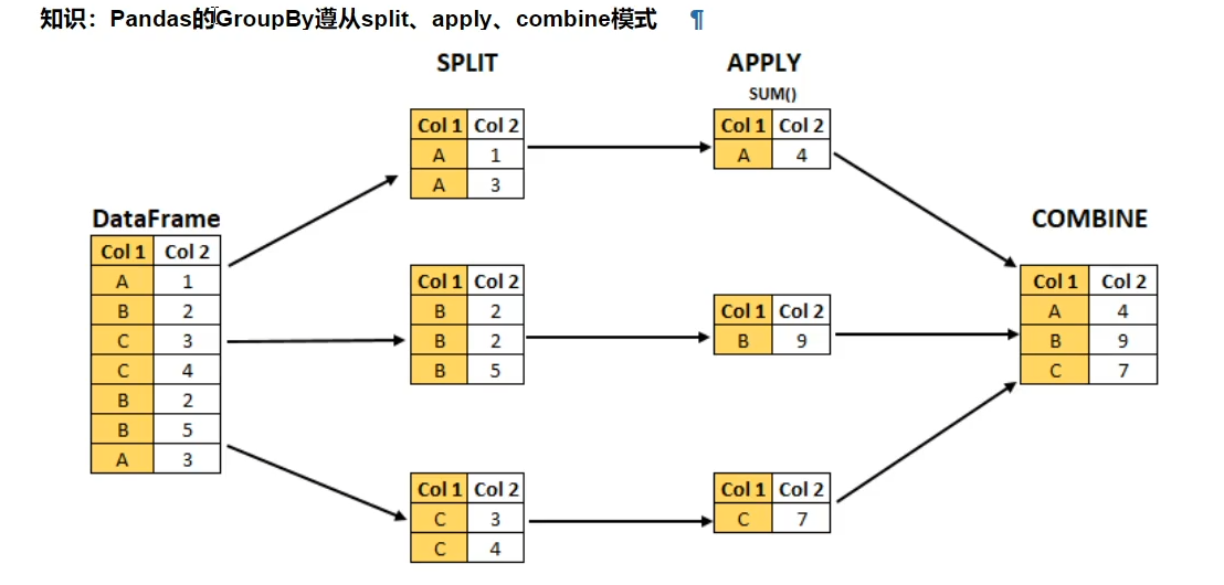
pandas 分组统计
pandas 实现groupby 分组统计
python
import pandas as pd
import numpy as np
# %matplotlib inline 是一个 Jupyter Notebook 的魔法命令,用于在 Notebook 中内嵌绘制图形。
%matplotlib inline

df = pd.DataFrame({'A':['foo', 'bar', 'foo', 'bar', 'foo', 'bar','foo', 'foo'],
                  'B':['one', 'one', 'two', 'three', 'two', 'two','one', 'three'],
                  'C':np.random.randn(8),
                  'D':np.random.randn(8)})
df
df.dtypes
A object
B object
C float64
D float64
dtype: object
分组使用聚合函数做数据库统计
python
# 1. 单个列groupby, 查询所有数据列的统计
df.groupby('A').sum()

# 注意:不难看出,新版本的groupby 语法中,开始不再忽略ouject 字符串数据,后面学习使用相关统计语句需要注意,以免发生错误| B | C | D | |
|---|---|---|---|
| A | |||
| bar | onethreetwo | -2.607356 | 1.918064 |
| foo | onetwotwoonethree | -0.650488 | 0.407203 |
python
# 2. 多个列groupby, 查询所有数据列的统计
df.groupby(['A', 'B']).mean() # 通过输出可以发现 AB 成对变成了二级索引| C | D | ||
|---|---|---|---|
| A | B | ||
| bar | one | -0.779027 | 1.223204 |
| three | -0.225912 | 0.488460 | |
| two | -1.602417 | 0.206401 | |
| foo | one | -0.093822 | 0.337233 |
| three | -0.996514 | 0.260899 | |
| two | 0.266835 | -0.264081 |
python
#避免变成索引的解决方案
df.groupby(['A', 'B'], as_index=False).mean()
python
# 3. 同时查看多种数据统计
# 删除 B 列
df_without_B = df.drop(columns=['B'])
df_without_B.groupby('A').agg(["sum", "mean", "std"])| C | D | |||||
|---|---|---|---|---|---|---|
| sum | mean | std | sum | mean | std | |
| A | ||||||
| bar | -3.405324 | -1.135108 | 0.689675 | -1.790008 | -0.596669 | 1.009874 |
| foo | -0.187476 | -0.037495 | 0.642890 | -1.830050 | -0.366010 | 1.197339 |
python
# 4. 查看单列结果数据统计
# 方法1
df.groupby('A')['C'].agg(["sum", "mean", "std"])
# 方法2
df_without_B.groupby('A').agg(["sum", "mean", "std"])['C'] # 以A列进行分组 进行统计 选出C列| sum | mean | std | |
|---|---|---|---|
| A | |||
| bar | -3.405324 | -1.135108 | 0.689675 |
| foo | -0.187476 | -0.037495 | 0.642890 |
python
# 5. 不同列使用不同的聚合函数
df.groupby('A').agg({'C':'sum', 'D':'mean'})| C | D | |
|---|---|---|
| A | ||
| bar | -3.405324 | -0.596669 |
| foo | -0.187476 | -0.366010 |
遍历groupby 的结果理解执行流程
python
# 1. 遍历单个列聚合的分组
g = df.groupby('A')
g
<pandas.core.groupby.generic.DataFrameGroupBy object at 0x00000287A0D73910>
python
for name, group in g:  # 遍历g  并将名称 和 值分别赋予给 name 和group
    print(name)
    print(group)
    print()
bar
A B C D
1 bar one -1.753535 0.172491
3 bar three -1.260420 -1.740289
5 bar two -0.391369 -0.222210
foo
A B C D
0 foo one -0.124441 -1.483866
2 foo two 0.950794 1.587760
4 foo two -0.419235 -0.962665
6 foo one 0.143290 -0.861839
7 foo three -0.737884 -0.109441
python
# 获取单个分组数据
g.get_group('bar')| A | B | C | D | |
|---|---|---|---|---|
| 1 | bar | one | -1.753535 | 0.172491 |
| 3 | bar | three | -1.260420 | -1.740289 |
| 5 | bar | two | -0.391369 | -0.222210 |
python
# 遍历多个列聚合的分组
g = df.groupby(['A', 'B'])
for name, group in g:  # 遍历g  并将名称 和 值分别赋予给 name 和group
    print(name)
    print(group)
    print()
# 输出结果可以看到 name 是一个2个元素的tuple ,代表不同的列
('bar', 'one')
A B C D
1 bar one -1.753535 0.172491
('bar', 'three')
A B C D
3 bar three -1.26042 -1.740289
('bar', 'two')
A B C D
5 bar two -0.391369 -0.22221
('foo', 'one')
A B C D
0 foo one -0.124441 -1.483866
6 foo one 0.143290 -0.861839
('foo', 'three')
A B C D
7 foo three -0.737884 -0.109441
('foo', 'two')
A B C D
2 foo two 0.950794 1.587760
4 foo two -0.419235 -0.962665
python
# 查询特定值对应的group 数组
g.get_group(('foo', 'one'))| A | B | C | D | |
|---|---|---|---|---|
| 0 | foo | one | -0.124441 | -1.483866 |
| 6 | foo | one | 0.143290 | -0.861839 |
案例: 分组探索天气数据
python
# 阅读天气数据源文件
fpath = "xxx.wether_data.csv"
df = pd.read_csv(fpath)
# 替换温度后缀 ℃
df.loc[:, "hwendu"] = df["hwendu"].str.replace("C","").astype('int32')
df.loc[:, "lwendu"] = df["lwendu"].str.replace("C","").astype('int32')
# 新增一列为月份
df['month'] = df['ymd'].str[:7] # 对ymd中的数据的前七个字符进行切片 并将结果赋值给month   2018-01-01 --->2018-01

# 案例1: 查看每个月的最高温度
data= df.groupby('month')['hwendu'].max()
data.plot()    # 画图  横坐标为月份 纵坐标为温度

# 案例1: 查看每个月的最高温度、最低温度、平均空气质量指数
group_data = df.groupby('month').agg('hwendu':'max', 'lwendu':'min','aqi':'mean')
group_data.plot()
pandas的 数据转换函数 map apply applymap
map 实现每个值对每个值的映射
apply: series:每个值的处理 DF:每个轴的处理
applymap:(已被弃用)
python
# 公司股票代码到中文的映射  注意,这里是小写  所以要用lower 语法将公司列的值变为小写
dict_company_names = {
    "baidu" :"百度",
    "baba":"阿里巴巴",
    "iqy": "爱奇艺",
    "jd":"京东"
}

stock_history = pd.read_csv('./quotefile/股票历史数据.csv')
# 方法1 Series.map(dict)
stock_history['公司MD'] = stock_history["公司"].str.lower().map(dict_company_names)
stock_history

# 方法2 Series.map(funcation)      funcation的参数是Series的每个元素的值
stock_history["公司MF"] = stock_history["公司"].map(lambda x : dict_company_names[x. lower()])  # 公司力的值 传递给函数x
stock_history

# Series.apply(funcation)
stock_history['公司AF'] = stock_history["公司"].apply(lambda x: dict_company_names[x. lower()])

# DataFrame.apply(funcation)
stock_history['公司DF'] = stock_history.apply(lambda x: dict_company_names[x['公司']. lower()], axis=1)  # 此处的x指代整个DF
stock_history

#applymap 用于DataFrame 所有值的转换
sub_df = stock_history[['收盘', '开盘', '高','低', '交易量']]   # 筛选出五列并赋值给新的DF
    # 数字取整 并应用于所有函数
sub_df.map(lambda x: int(x))

# 直接修改stock_history 的值类型
stock_history.loc[:, ['收盘', '开盘', '高','低', '交易量']] = sub_df.map(lambda x: int(x))
stock_history| 日期 | 公司 | 收盘 | 开盘 | 高 | 低 | 交易量 | 涨跌幅 | 公司MD | 公司MF | 公司AF | 公司DF | |
|---|---|---|---|---|---|---|---|---|---|---|---|---|
| 0 | 2024/3/22 | IQY | 4.0 | 4.0 | 4.0 | 3.0 | 7.0 | -0.0074 | 爱奇艺 | 爱奇艺 | 爱奇艺 | 爱奇艺 |
| 1 | 2024/3/21 | IQY | 4.0 | 4.0 | 4.0 | 4.0 | 5.0 | -0.0216 | 爱奇艺 | 爱奇艺 | 爱奇艺 | 爱奇艺 |
| 2 | 2024/3/20 | IQY | 4.0 | 4.0 | 4.0 | 3.0 | 6.0 | 0.0532 | 爱奇艺 | 爱奇艺 | 爱奇艺 | 爱奇艺 |
| 3 | 2024/3/19 | IQY | 3.0 | 3.0 | 3.0 | 3.0 | 5.0 | -0.0075 | 爱奇艺 | 爱奇艺 | 爱奇艺 | 爱奇艺 |
| 4 | 2024/3/18 | IQY | 3.0 | 4.0 | 4.0 | 3.0 | 5.0 | -0.0050 | 爱奇艺 | 爱奇艺 | 爱奇艺 | 爱奇艺 |
| ... | ... | ... | ... | ... | ... | ... | ... | ... | ... | ... | ... | ... |
| 75 | 2024/3/1 | JD | 23.0 | 23.0 | 23.0 | 22.0 | 13.0 | 0.0168 | 京东 | 京东 | 京东 | 京东 |
| 76 | 2024/2/29 | JD | 22.0 | 22.0 | 23.0 | 22.0 | 14.0 | -0.0083 | 京东 | 京东 | 京东 | 京东 |
| 77 | 2024/2/28 | JD | 22.0 | 23.0 | 23.0 | 22.0 | 15.0 | -0.0527 | 京东 | 京东 | 京东 | 京东 |
| 78 | 2024/2/27 | JD | 24.0 | 24.0 | 24.0 | 23.0 | 9.0 | 0.0160 | 京东 | 京东 | 京东 | 京东 |
| 79 | 2024/2/26 | JD | 23.0 | 23.0 | 24.0 | 23.0 | 6.0 | -0.0084 | 京东 | 京东 | 京东 | 京东 |
80 rows × 12 columns
pandas对每个分组应用apply 函数
归一化公式
y = (x-最小值)/最大值 - 最小值
案例 对评分数据进行归一化
python
# 实现按照用户ID进行分组, 然后对其中一列进行归一化
def ratings_norm(df):
    # @df: 每个用户分组的DataFrame

    min_value = df['rating'].min()
    max_value = df['rating'].max()
    df["ratings_norm"] = df["rating"].apply(lambda x: (x-min_value)/max_value-min_value)
    return df

ratings = ratings.groupby("userID").apply(ratings_norm)
pandas 使用stack 和pivot 实现数据透视
python
> **案例: 统计得到电影评分数据集,每个月份的每个分数被评分多少次:(月份,分数1~5,次数)**python
df_movie_rating = pd.read_csv(xxx.csv)  # 表头包含  UserID  MovieID  Rating  Timestamp(时间戳)

#step1 日期处理
df_movie_rating['pdate'] = pd.to_datetime(df_movie_rating["df_movie_rating"], unit ='s')
# 实现数据统计
df_group = df.groupby([df['pdate'].dt.month, "Rating"])["UserID"].agg(pv=sum)   # 用日期 和rating作为列  px:一个新的列的名称
#  此方法缺点:想查看按月份 不同评分的次数趋势 是没法实现的

# Step2 使用 unstack 实现数据的二维透视(升唯)    目的: 想要画图对比按照月份的不同评分的数量趋势
df_stack = df_group.unstack()
df_stack.plot

# unstack 和stack 是互逆操作  行和列进行互转
# 使用 pivot  简化透视
df_reset = df_group.reset_index()  # 重溅索引
df_pivot = df_reset.pivot('pdate', 'Rating','pv')
python
# **19 pandas 使用apply 函数给表格同时添加多列**